Over the last few years, researchers have applied deep learning to all sorts of datasets in biology and medicine. On almost every problem – from identifying protein-DNA interactions to diagnosing Alzheimer’s disease from brain scans – deep learning techniques have performed remarkably well, leaving traditional machine learning in the dust.

These results are somewhat surprising – deep learning was inspired by the architecture of the human nervous system, which explains why it works so well on conventional, “human” tasks like image recognition and natural language processing. But what about tasks like sifting through large amounts of DNA sequences and identifying sites that bind to proteins – why do neural networks perform so well?

In this post, I examine 4 fundamental deep learning architectures, and consider why they are suited to solving problems in medicine and functional genomics. But before that, let’s start with machine learning basics.

Preliminaries

Machine learning is pattern recognition. Historically, the earliest patterns that computers were tasked to recognize were linear patterns that mapped input data, represented in the form of feature vectors, to output data, represented as discrete or continuous scalar labels. Linear models can only describe certain kinds of datasets, and so a long time ago, researchers found ways of transforming non-linear relationships into linear ones, which were then easily tackled by standard linear machine learning algorithms. However, these approaches required knowing (or guessing) the explicit non-linear relationships between the input data and output data, and “hand-engineering” features to remove these non-linearities.

The focus of this guide is not on these traditional approaches, but on deep learning and its corresponding architecture, deep neural networks.

The beauty and power of deep neural networks (or “nets”) is that computers are made to guess the nonlinear relationships within the dataset on their own. The beauty is the simplicity: just as a typical machine learning method iteratively guesses the linear weights that maps inputs to outputs, neural networks iteratively guess the nonlinear function that best map the inputs to the outputs. The difference, of course, is that the set of nonlinear functions that could possibly map inputs to outputs is much larger than the set of linear functions.

So how do neural networks do it? Can neural networks really really find any possible non-linear function that relates inputs and outputs? It turns out that the answer is yes, a standard neural network with just 1 hidden layer (more on that layer later) can approximate any continuous, non-linear function! This is a useful theoretical result, but practically speaking, it doesn’t mean much, as the theorem says nothing about the computation time or memory required to perform this approximation for an arbitrary function.

Yet it turns out that most “real-world” non-linear datasets are characterized by certain properties that are well-suited to learning by deep neural nets, meaning that neural net-based algorithms are highly efficient in capturing patterns within those datasets. Although it is not necessary to know these properties to use neural nets, it is interesting to think about how these properties, such as locality and symmetry, connect to the fundamental physical processes that generate the data, as well as which properties are emphasized in each of the 4 architectures that we will discuss.

1. Feedforward, Fully-Connected Neural Networks

Let’s start by considering a classic problem in functional genomics.

Transcription Factor Binding: during transcription (the process in which DNA sequences are read and converted to RNA), a variety of proteins bind to the DNA molecule being transcribed. These proteins, called transcription factors, have different effects: some may promote the process of transcription, while others will inhibit it. It is of great interest to researchers to know exactly where (i.e. what part of the DNA sequence) a particular transcription factor will bind.

To learn this information, biologists can conduct experiments that provide “rough” answers: for example, a researcher might do an experiment with 500 DNA sequences, each consisting of 40 nucleotide bases (a typical 40-base sequence might be:

AATGCGGCCCGGTATTGACCAGGATTACGATCAGGTTTAG

where each of A, T, C, and G represents one base). We may learn through experiments that the transcription factor binds to the first 200 sequences very strongly, to the next 200 weakly, and not at all to the last 100 sequences. This gives us some information about DNA-protein binding, but doesn’t completely tells us where the protein binds, because the protein only requires a particular sequence of 4 or 5 bases (this is known as a motif) to bind to, and some small variations in the motif may be OK (the protein will still bind to the sequences, but not as strongly) while other variations in the motif may disrupt binding altogether. In addition, certain global properties (such as the percentage of bases that are C and G, known as the GC-content, in the sequence) may affect binding as well.

Given this dataset, how do we identify the motif (or motifs!) that the transcription factor binds most strongly to?

As a first pass, you might decide to frame this as a linear regression problem: given a matrix of 500 columns, where each column encodes 1 input sequence, and a vector of labels of length 500, where each label encodes the affinity of a sequence to the protein, what weight vector maps the input matrix to the output labels most closely? Such an approach is illustrated below (you can think of each base being represented by an integer: A=0, T=1, C=2, G=3, although there is a better way to encode categorical features):

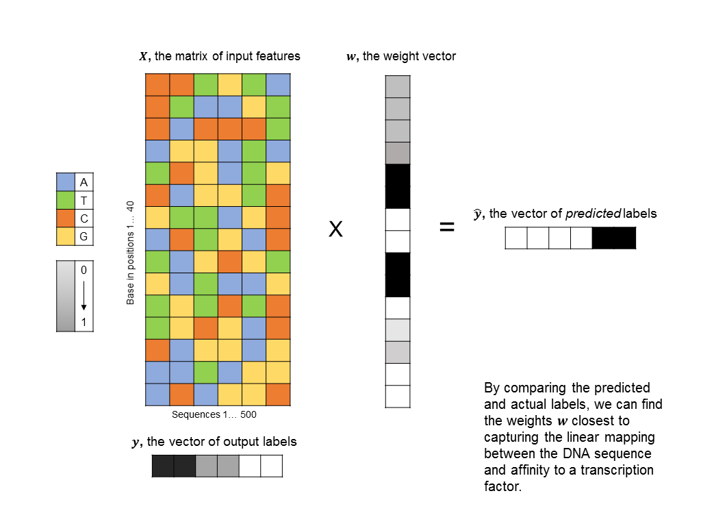
The problem with this formulation is that does not take into account any non-linearities in the relationship between input sequences and binding affinity. In particular, we’d like the algorithm to identify motifs, such as “CCGGT” that cause the transcription factor to bind. However, linear techniques

cannot have an “all-or-nothing” response. A transcription factor will probably not bind at all if it sees either a “CC” or “GGT” by itself, but will bind strongly if “CCGGT” appears together. However, a linear model will necessarily produce weak binding responses to “CC” and “GGT” if it is to produce a strong response to “CCGGT” cannot take into account proximity of bases. While it is possible to linearly model spatial dependence (a “C” at the beginning of the sequence counts different than “C” in the middle), it is not possible to weigh a “C” and a “G” together differently than a “C” and a “G” apart. This makes it virtually impossible to identify motifs, which have to occur together, or any other local phenomena. So, how do we extend our model to include these nonlinear relationships? In the traditional machine learning framework, you would do “feature engineering” – select features that capture the nonlinear nature of the problem you are interested in solving. For example, in this case, it might make sense to make each feature the number of times every possible 5-nucleotide sequence (“5-mer”) appears in the entire 40-nucleotide sequence.

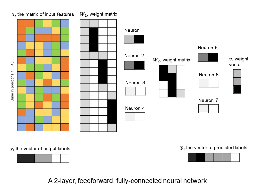
However, this requires a lot of thought and domain expertise. In the framework of deep learning, we instead create a bunch of neurons, each of which takes as input a linear combination of the original features. Then, each of these neurons activate, meaning that they output a value that is a non-linear function of their input. (The particular choice of non-linear function can vary, and won’t be discussed here). The output values can then be summed to produce a predicted label. This approach is shown here:

A layer of neurons is known as a hidden layer, as it does not directly represent the input, nor the output, but is an intermediary between the two. You might ask – what if we were to add another layer of intermediary neurons? Deep neural networks take this concept to heart, and can have many hidden layers of neurons that feed into each other before outputting a prediction value. Like this:

This allows them to capture more and more complex features. For example, the neurons in the first hidden layers might capture small motifs. The neurons in the second hidden layer might capture combinations of motifs, or global properties, like GC-content (although global properties could be captured in the first layer as well). And so on.

As an aside, it is worth mentioning that the idea of having more than 1 layer only makes sense with a nonlinear activation function. If we restrict ourselves to dealing with linear activation functions, adding multiple layers offers no advantage, since a linear function of a linear combination is still a linear combination. However, linear combinations of non-linear functions can produce non-linear functions that are not part of the original set of functions.

2. Convolutional Neural Networks

You’ll notice something interesting in the 2-layer neural network that I illustrated above. The first hidden layer consists of 4 neurons, but the weights that feed into neurons 2, 3, and 4 follow a particular pattern. Each neuron has the same set of weights, but these weights are applied to different parts of the input sequence.

It’s not surprising that the neural network has learned this pattern of weights, since (if trained on a good dataset,) it should learn to identify the same motif, wherever it may be in the sequence. Therefore, we might expect one neuron to search for the motif at the beginning of the beginning of the DNA sequence, another to search in the middle, and another near the end of the sequence.

If we already expect the weights to take this form, why not use a neural network architecture that requires all of our neurons in a given layer to learn the same weights, only translated across the input sequence? What’s the advantage of doing this? Because this significantly reduces the number of free parameters in our model, which in turn cuts down the computational time and memory, as well as reduces the chance of overfitting our data.

This kind of architecture is known as convolutional neural network, and a layer that enforces the constraint just described is known as a convolution layer. Again, the power of convolution layers is that they tend to pick the “right” patterns – those that repeat throughout our input features – all while having very few parameters that need to be learned. Here’s an example of a convolutional layer that tries to learn a 5-base motif anywhere in our input sequence.

You’ll notice that the number of free parameters in the convolutional layer is just 5, instead of the significantly bigger number in the first hidden layer of the fully-connected neural network above. Even the fully-connected layer that follows the convolutional layer usually has a simple structure (in our cases it is uniform, because it responds uniformly to matched motifs anywhere in the DNA sequence), so we can simplify it using a max pooling layer, which further reduces the number of parameters in the model. ConvNets are in fact the architecture used by a recent paper in Nature for predicting protein-DNA interactions.

3. Recurrent Neural Network

Now, let’s say your biologist friend comes along and tells you a little bit more about functional genomics.

Transcription factors are of different types: there are activators, which increase transcription when they bind to DNA, as well as repressors that decrease transcription activity when they bind. Both activators and repressors often bind close to the promoter region of the DNA squence, where transcription begins.

Because of the proximity of different kinds of protein-binding sites to each other, it may possible to make better predictions of whether a protein will bind to DNA, if we know where this DNA sequence is located, relative to other DNA sequences. For example, if we have just identified an activator-binding site in our DNA sequence, then the chance of identifying another activator-binding site closeby is higher.

Given this information, can we build a neural network architecture that better predicts which DNA sites will bind to a given transcription factor?

Now, we’re faced with a whole new type of problem, one that requires keeping track of what features have been identified in our sequence so far, and adjusting our prediction weights accordingly.

In the jargon of natural language processing, there is now a grammar to the DNA-protein binding problem, and taking this grammar into account requires a different way of thinking about processing data, one that is sequential, instead of singular. A neural network architecture that is suited to sequential inputs and outputs is the recurrent neural network (RNN).

A simple RNN is illustrated in the following graphic. There are two fundamental differences between this RNN and the feedforward neural nets we saw earlier. 1) We are training many DNA sequences, one after another, and there is a sequential relationship between each set of input features 2) a memory unit is introduced that stores the state of the RNN and which is updated at every step in the sequence.

The architecture shown here is often described as a “vanilla RNN” because it is probably the simplest way you could incorporate memory into a neural network. It has some shortcomings, such as the fact that the RNN does not retain any long-term memory (the memory vector only affects the very next output). To address this shortcoming, the long short-term memory (LSTM) architecture is often used to improve accuracy and stability.

A recent paper in functional genomics used a combined CNN-RNN architecture with LSTM units to achieve breakthrough performance in protein-DNA binding prediction.

4. Autoencoders

Let’s shift gears and look at a different problem: diagnosing autism based solely on brain scans.

Diagnosing Autism: currently, the standard way of diagnosing autism spectrum disorder (ASD) in children is through a series of behavioral evaluations performed by trained psychologists and clinicians. However, these tests by their nature leave room for human subjectivity.

Many studies have noted that patients with ASD exhibit certain unusual variations in neurological activity. This raises the question: can we diagnose ASD based solely on scans of the brain, such those taken with functional magnetic resonance imaging (fMRI)?

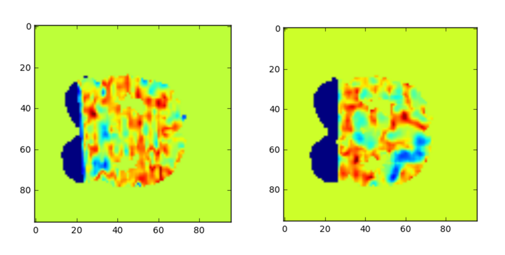
Here are two fMRIs, one taken from a subject with ASD and one without, taken from the ABIDE dataset.

Classifying which fMRI belongs to which subject falls into the category of image recognition, and a ConvNet is well-suited to the task. However, there’s a problem - each of these brain scans generally consists of over a million voxels. Yet, it hard to generate even a few hundred clean images to train our ConvNet. Because the number of features vastly outnumbers the number of training examples, we are likely to overfit our model, even with a convolutional neural network.

To address this problem, note that many of the voxels in the fMRIs are either blank or are similar to neighboring voxels. So, we might consider first compressing our input images into a representation that consists of fewer features. In other words, we map our highly-dimensional images into a lower-dimensional space, which we can then classify more easily.

How do we know if we have a good mapping into a lower dimension? There are plenty of lower-dimensional representations that lose too much information. For example, I could multiply all of the pixel values in my original image by zero to obtain a very sparse representation. But clearly, this representation is terrible. A good way to measure how much information is lost is to see how well we can reconstruct our original image from the compressed representation.

With this in mind, we can construct an autoencoder neural network that tries to minimize the difference between the original input image and one that has been compressed and then reconstructed:

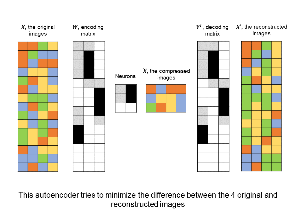
Unlike other architectures above, this is an unsupervised neural network. Instead of trying to minimize the difference between predicted and actual labels, there are no labels at all, and instead, the difference between input images and reconstructed images.

Once we have found a compressed representation, then we can feed that into a convolutional neural network to perform the classification between patients with autism and those without autism.

Conclusion

When analyzing datasets in medicine and biology there is surprisingly often a neural network architecture that is well-suited to the application. Although neural networks are often toted as “blind machine learning” – in that they can be applied without any domain expertise – we’ve seen how knowing something about the biology underlying a problem can help find the right architecture.