Today, I spent some understanding the Expectation-Maximization (EM) algorithm. It was the 8th or 9th time I had tried to understand it, because even though there are many nice tutorials about it online, about three quarters of the way through them, my eyes start to glaze over the math, and I end up leaving with only a “high-level understanding” of the algorithm. Today, I think I truly get it, and I’m going to try to explain it in a way that would have been clearest to me from the beginning. I’ve divided this article into 3 passes, each of which provide an understanding of the algorithm from a different perspective.

Pass 1: Intuition

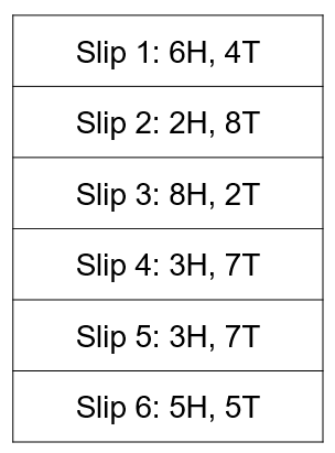
Suppose you have two friends, Ali and Bilal, each of whom have a biased coin that flips heads with probabilities \(a\) and \(b\) respectively. They flip their coins 10 times and write down the number of heads and tails they get on a slip of paper. They repeat this process several times, generating many slips of papers, which they stuff into an envelope and hand it to you. Based only on the numbers written on the slips of paper, can you estimate the original probabilities \(\{a,b\}\)? (The order of \(a\) and \(b\) doesn’t matter, just their values.)

So how might you approach this problem?

(1) Well, if there was only one person, say Ali, writing down numbers, then this would be a very simple question. You would simply count the number of heads and divide it by the total number of flips of the coin. In the example above, if Ali generated all 6 slips, then your estimate of \(a\) would be:

\[\frac{(6+2+8+3+3+5)}{60} = 0.45\]

Your intuition likely tells you that this strategy will give you a good estimate of \(a\). In fact, this is the maximum likelihood estimate (MLE) of \(a\), defined as the value of \(a\) that produces the highest probability of observing the given data, and it is consistent, meaning that with enough slips of paper, you can estimate \(a\) to any desired degree of accuracy.

(2) However, the tricky thing in this problem is that you have two separate coins with their own biases, and you don’t know whether each slip of paper is comes from Ali’s coin or Bilal’s. If you knew the assignment of the slips to either Ali or Bilal (e.g. if they each handed you a separate envelope), then you could carry out the procedure in (1) separately for Ali and Bilal, and this problem would be a piece of cake. (This is a common feature of EM problems: if you knew some “hidden variables”, producing an estimate would be super easy.)

(3) But all hope is not lost. Looking at the example above, it seems that the slips belong to two clusters, one that produces flips with a low frequency of heads (slips 2, 4, and 5) and another sets of slips that seem to come from a coin that lands on heads more often (slips 1, 3, and 6). It seems natural to think that one set of slips corresponds to Ali and the other to Bilal. We could make this assumption and then calculate the MLE estimate of \(a\) and \(b\), just like we did before:

\[\begin{align*} \text{Estimate of}\; a = \frac{6+8+5}{10} = 0.63\\ \text{Estimate of}\; b = \frac{2+3+3}{10} = 0.27 \end{align*}\]

(4) But, what if we’re wrong? Maybe instead, both coins are actually fair, and all of the observed variation is simply due to chance. How do we know which case is correct? To decide between various options for \(a\) and \(b\), we should compute the probability that our data would be generated under that assumption, and choose the values of \(a\) and \(b\) that has the highest probability of occurring. So for example, if \(a=0.3, b=0.9\), then slip 4 (with 3H, 7T) could have been generated by Ali with a high probability and by Bilal with a low probability. We would average those together to get net likelihood of observing slip 4, and then we would repeat this process for every slip, and multiply those likelihoods together to get the probability of observing all of the data in the envelope. The values of \(a\) and \(b\) that maximize this probability is, again, called the maximum likelihood estimate.

(5) The only problem with this approach is that there are an infinite number of values to guess for \(a\) and \(b\), and unlike the situation described in (1), it’s not immediately clear how to select these parameters to maximize the likelihood. An alternative strategy might be to guess an assignment of slips to Ali and Bilal, since there are only a finite number of ways to assign the slips. For each assignment, we compute the MLE estimate of \(a\) and \(b\), and we choose the assignment that maximizes the probability of observing all of the data. Even though this is a better strategy, it is still exponential in the number of slips, \(N\), since there are \(2^N\) assignments…

(6) Well, what if we start with a random assignment and even if we’re wrong, we don’t start over from scratch, but just reallocate slips in a way to make the likelihood higher based on our initial assignment? For example, suppose we start by allocating slips 1, 2, and 3 to Ali, and slips 4, 5, and 6 to Bilal. Then, our MLE estimate of \(a\) would be 0.53 and \(b\) would be 0.37. Under these values of \(a\) and \(b\), it is much more likely that slip 2 was actually generated by Bilal and slip 6 by Ali, so in the next iteration, we assign slips 1, 3, and 6 to Ali, and slips 2, 4, and 5 to Bilal. For slips that we are not sure about, we could even “partially” allocate them to Ali and “partially” to Bilal. Then, based on the new allocation, we recompute the MLE estimates of \(a\) and \(b\), and continue to iterate in this fashion.

---

This is the basic idea behind the Expectation-Maximization (EM) aglorithm. It consists of two steps, that are repeatedly performed:

E-step: Compute the expected value of your “hidden variables” (in this case, the assignment of slips to people), based on the current values of the parameters.

M-step: Recompute the most likely value of your parameters based on the value of the hidden parameters and the observed data.

Implicit in this formulation is that the “hidden variables” should be chosen in a problem-specific manner so that the M-step can be performed easily.

OK so this may seem like a reasonable strategy, but there are two important questions that need to be answered:

• Question 1: Is this process of iterative improvement guaranteed to improve the likelihood? In other worse, can we be sure end up that by reassigning the labels and recalculating \(a\) and \(b\), we never reach values that are less likely to produce the observed data?
• Question 2: Is this process guaranteed to eventually reach the estimate with the highest likelihood (the global MLE)?

We answer these questions in Pass 2 and Pass 3 respectively. It turns out that the answer to the first is “yes”, while the second is “no”, meaning that EM guarantees convergence, but not necessarily to the global optima.

Pass 2: Math

In order to prove some guarantees about EM, we do need to do some math. I’ll try make the notation and derivation as natural as possible.

Let \(\theta\) be the variable we use to refer to all of the parameters that we are maximizing (in the above example: \(a\) and \(b\)). The estimate of the parameters on the \(n^\text{th}\) step, we will denote as \(\hat{\theta}_n\).

We would like to find the parameters that maximize the probability of our observations, which we’ll denote as realizations of a random variable, \(X\). We will treat the “hidden variables” as realizations of a random variable, \(Z\). (We will abuse notation a little bit and use these letters to refer to both the random variables and their realizations.)

Thus, Question 1 basically asks whether it is guaranteed that:

\[p(X|\hat{\theta}_{n+1}) \ge p(X|\hat{\theta}_n),\]

i.e. that the parameter estimates at step \(n+1\) have a higher likelihood than the parameter estimates at step \(n\). Because \(\ln \) is a monotonically increasing function, we can actually write this in terms of the log-likelihoods, which will be easier to work with:

\[\ln p(X|\hat{\theta}_{n+1}) \ge \ln p(X|\hat{\theta}_n), \tag{1}\label{eq:1}\]

To determine whether \eqref{eq:1} is true, we need to know how \(\hat{\theta}_{n+1}\) is related to \(\hat{\theta}_{n}\). So, let us remember how \(\hat{\theta}_{n+1}\) is defined. Combining both the E-step and M-step together in one equation, we have:

\[\begin{align*} \hat{\theta}_{n+1} &= \arg \max_{\theta} \mathbb{E}[ \ln p(X,Z|\theta)] \tag{2}\label{eq:2} \end{align*}\]

A couple of things to note here: First, we have changed things a little from the E-step described earlier, so that we are maximizing the expected log-likelihood instead of the expected likelihood, as this will simplify the math. Second, the expectation in \eqref{eq:2} is over \(Z|X,\hat{\theta}_n\), i.e. we weight every term in the expectation by how likely the assignment is, \(p(Z|X,\hat{\theta}_n)\). More explicitly, we rewrite \eqref{eq:2} as:

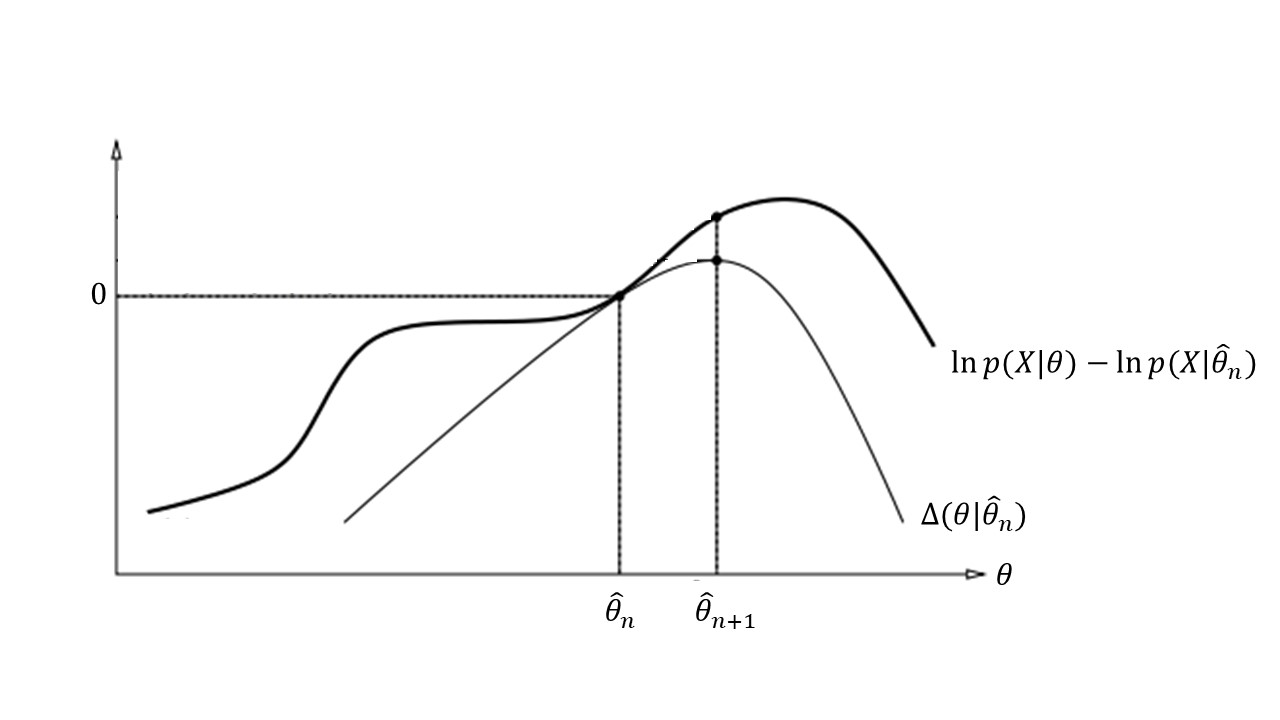
\[\begin{align*} \hat{\theta}_{n+1} &= \arg \max_{\theta} \sum_Z p(Z|X,\hat{\theta}_n) \ln{p(X,Z|\theta)} \\ &= \arg \max_{\theta} \sum_Z p(Z|X,\hat{\theta}_n) \ln \frac{ p(X,Z|\theta)}{p(X,Z|\hat{\theta}_n)} \tag{3}\label{eq:3} \\ &\stackrel{def}{=} \arg \max_{\theta} \Delta(\theta|\hat{\theta}_n) \end{align*}\]

Here, we are allowed to go from the first line to the second, since we have only introduced a term that is independent of \(\theta\), so it doesn’t change the result of \(\arg \max\). Of course, that doesn’t explain why it would be a good idea to do this particular algebraic manipulation. To motivate that, notice that this new function that we have defined has a special property, namely:

\[\Delta(\hat{\theta}_n|\hat{\theta}_n) = 0, \tag{4}\label{eq:4}\]

since \(\ln{1}=0\). Thus, \(\Delta(\hat{\theta}_{n+1}|\hat{\theta}_n)\) must be at least \(0\), because \(\hat{\theta}_{n+1}\) is chosen with the express purpose of maximizing this quantity.

Now, wouldn’t it be great if \(\Delta(\hat{\theta}_{n+1}|\hat{\theta}_n)\) was equal to \(\ln p(X|\hat{\theta}_{n+1}) - \ln p(X|\hat{\theta}_n) \)? Because then, \eqref{eq:1} would follow from the previous paragraph. (Go back and convince yourself that this is true.)

But of course, it can’t be so simple. If that was the case, then maximizing \(\Delta(\theta|\theta_n)\), which is usually easy to do, would directly give us the MLE estimate of \(\theta\) in one step, instead of the iterative procedure that EM requires. It turns out that have the next best thing. As we will the prove below, the following is true:

\[\ln p(X|\theta) - \ln p(X|\hat{\theta}_n) \ge \Delta(\theta|\hat{\theta}_n) \tag{5}\label{eq:5}\]

Once we have shown that this is true, we have proven that the EM algorithm can only improve (or leave the same) the log-likelihood of the estimated parameters. Why? Because of these three facts taken together:

• At each step of EM, the “delta” function is non-negative: \(\Delta(\hat{\theta}_{n+1}|\hat{\theta}_n) \ge 0\),
• If we had not changed the value of theta from step \(n\) to step \(n+1\), then the delta function would be zero, as would the difference in the log-likelihoods: \(\ln p(X|\hat{\theta}_{n+1}) - \ln p(X|\hat{\theta}_n)\)
• For all possible \(\hat{\theta}_{n+1}\), the difference in the log-likelihoods is greater than or equal to the “delta” function

… therefore, the difference in the log-likelihoods must always be non-negative. This is the key step in the proof, so it’s worth taking a minute to make sure that’s you’re convinced. The picture below illustrates this point:

The rest of the math is just algebra to prove \eqref{eq:5}:

\[\begin{align*} \ln p(X|\theta) - \ln p(X|\hat{\theta}_n) &= \ln \sum_Z p(X,Z|\theta) - \ln p(X|\hat{\theta}_n) \\ &= \ln \sum_Z p(X|Z,\theta) p(Z|\theta) - \ln p(X|\hat{\theta}_n) \\ &= \ln \sum_Z p(X|Z,\theta) p(Z|\theta) \frac{p(Z|X,\hat{\theta}_n)}{p(Z|X,\theta_n)} - \ln p(X|\hat{\theta}_n) \\ &= \ln \sum_Z p(Z|X,\hat{\theta}_n) \frac{p(X|Z,\theta) p(Z|\theta)}{p(Z|X,\hat{\theta}_n)} - \ln p(X|\hat{\theta}_n) \\ &\ge \sum_Z p(Z|X,\hat{\theta}_n) \ln \frac{p(X|Z,\theta)p(Z|\theta)}{p(Z|X,\hat{\theta}_n)} - \ln p(X|\hat{\theta}_n) \\ &= \sum_Z p(Z|X,\hat{\theta}_n) \ln \frac{p(X|Z,\theta)p(Z|\theta)}{p(Z|X,\hat{\theta}_n)p(X|\hat{\theta}_n)} \\ &= \sum_Z p(Z|X,\hat{\theta}_n) \ln \frac{p(X,Z|\theta)}{p(X,Z|,\hat{\theta}_n)} \\ &= \Delta{\theta|\hat{\theta}_n} \\ \end{align*}\]

The inequality on the fifth line follows from the fact that the natural log of a weighted sum of numbers is greater than the weighted sum of the natural log of those numbers, a consequence of Jensen’s inequality and the fact that the natural log is a concave function.

Pass 3: Simulation

We’ve shown that successive iterations in the EM algorithm can never decrease the log-likelihood of the parameter estimates. This means that EM will eventually converge to a particular value of the estimates, call it \(\theta^{*}\). Is \(\theta^{*}\) guaranteed to be maximum likelihood estimate of \(\theta\)? The answer is generally no.

Perhaps the easiest way to see this is to do a simulation to visualize how the parameters evolve during an iteration of EM. Here, I have simulated EM with the experimental that I described in Pass 1 using two different initial values: \((a,b)=(0.05, 0.2)\) and \((a,b)=(0.1, 0.1)\). Take a look at the results (or see the python notebook):

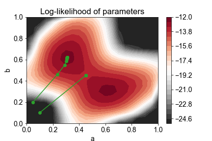
We see that the parameters improve, or at least stay the same, at every iteration of EM. However, EM does not guarantee that the globally optimal value of \(\theta\) is reached.

In practice, people perform the EM algorithm with multiple initial values, and hope that one of them will reach the globally optimal value, which usually works well!

---

Credit: adapted from a nice tutorial from the CS Department at the University of Utah.

---